Announcing Results from Aster's Autonomous Research System
Aster
We're releasing the first results from our autonomous research system. We cover
three benchmarks: Andrej Karpathy's NanoChat, ProteinGym, and the NanoGPT
speedrun.
Our system takes a problem, identifies promising research directions, and
launches parallel subagents to explore each hypothesis. The system can run
thousands of concurrent agents at once. The current version is already strong,
and we're excited about the breakthroughs still ahead.
Here is the link to our repository
with all results.
Andrej Karpathy's NanoChat
NanoChat Autoresearch: best validation BPB over wall-clock time (Aster vs. Recursive, Karpathy, and SkyPilot; lower is better). Annotations mark the modifications Aster discovered en route to 0.9098.
NanoChat, Karpathy's open-source repository, has become a popular proofpoint for
autonomous research systems — including the AutoResearch leaderboard, which has
drawn significant attention in the ML community.
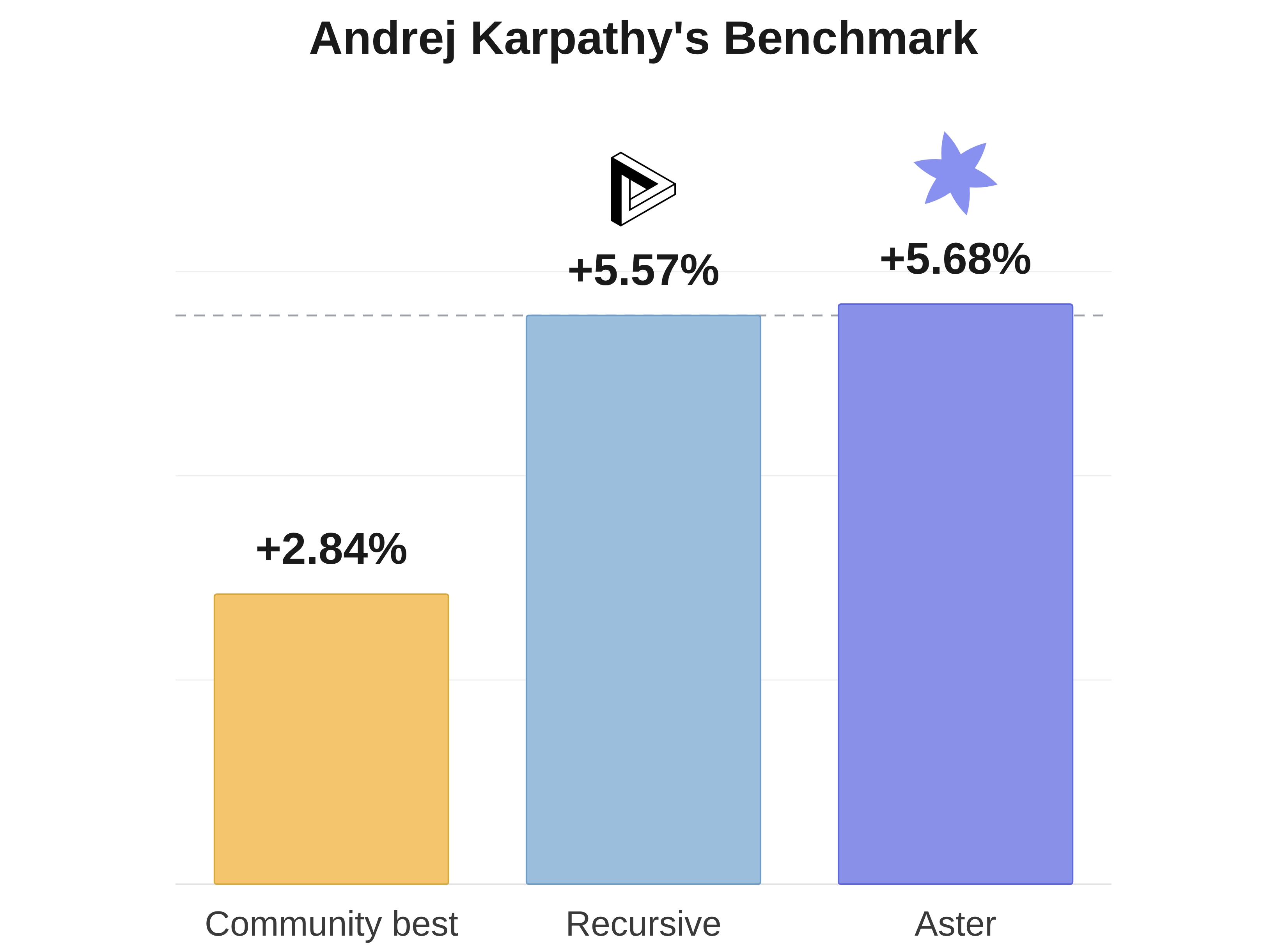
The best community-discovered result on AutoResearch reached 0.9372 BPB. A week
ago, another company shared results from their system: 0.9109 BPB after a
40-hour run.
Using our system, we found a solution at 0.9098 BPB. Within an hour, it had
already surpassed Karpathy's original overnight run. We parallelized across 30
B200s and ran for roughly 50 hours.
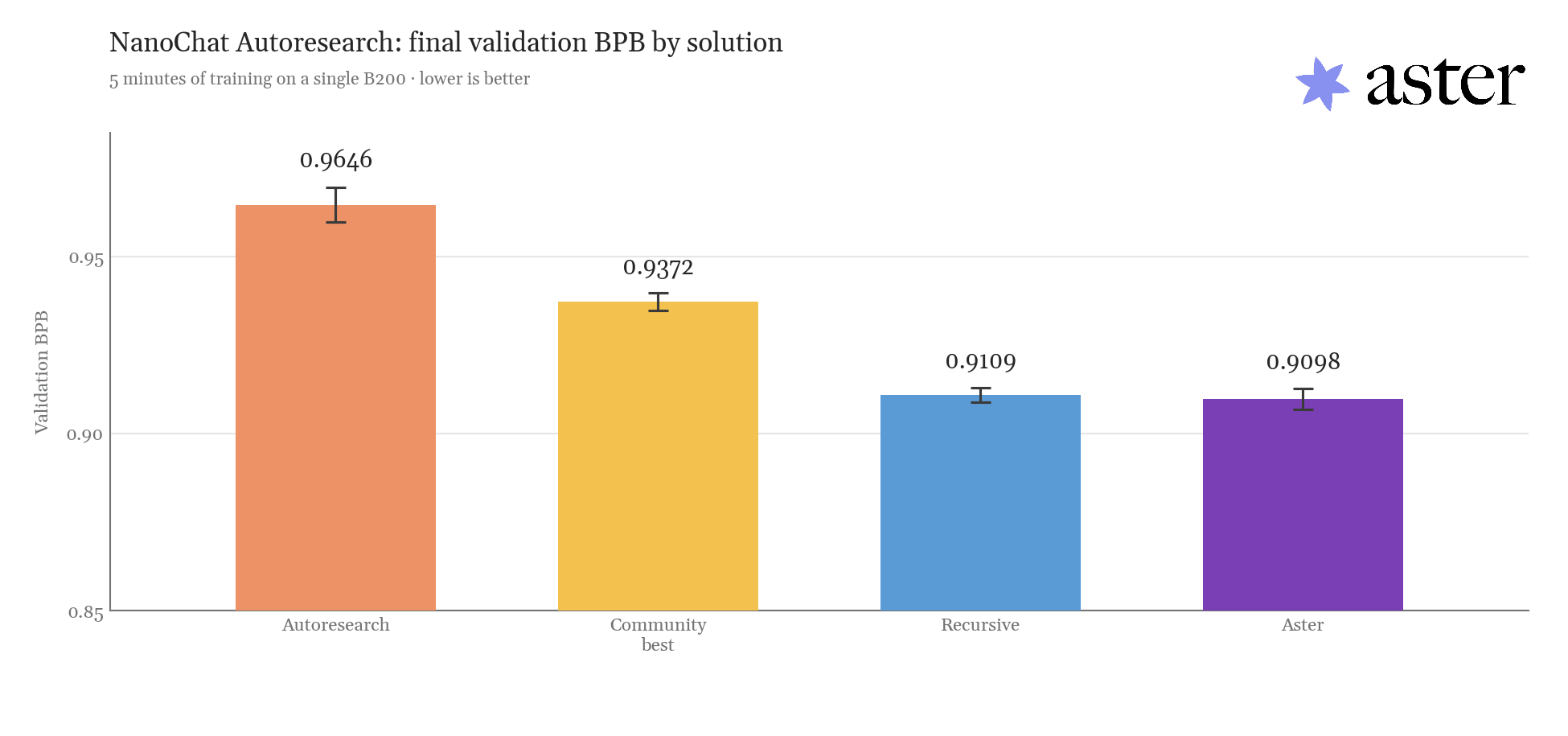
Final validation BPB by solution after five minutes of training on a single B200 (lower is better, 10-seed mean). Aster reaches 0.9098.
Here are a few of the modifications we found most interesting.
Triton Kernels
Aster folded the per-head RMS magnitude-decoupling and the gain into one Triton
kernel, roughly halving HBM traffic on the largest epilogue tensor while staying
numerically equivalent to the eager path.
_epi_configs = [ triton.Config({'BLOCK': 8}, num_warps=4), triton.Config({'BLOCK': 16}, num_warps=4), triton.Config({'BLOCK': 16}, num_warps=8), triton.Config({'BLOCK': 32}, num_warps=8),]@triton.autotune(configs=_epi_configs, key=['N'])@triton.jitdef _attn_epi_fwd_kernel(X, G, Y, N, eps, D: tl.constexpr, BLOCK: tl.constexpr): pid = tl.program_id(0) rows = pid * BLOCK + tl.arange(0, BLOCK) mask = rows < N safe = tl.where(mask, rows, 0) cols = tl.arange(0, D) off = safe[:, None] * D + cols[None, :] m2 = mask[:, None] x = tl.load(X + off, mask=m2, other=0.0).to(tl.float32) g = tl.load(G + safe, mask=mask, other=0.0).to(tl.float32) ms = tl.sum(x * x, axis=1) / D inv = g / tl.sqrt(ms + eps) tl.store(Y + off, (x * inv[:, None]).to(Y.dtype.element_ty), mask=m2)@triton.autotune(configs=_epi_configs, key=['N'])@triton.jitdef _attn_epi_bwd_kernel(X, G, GY, DX, DG, N, eps, D: tl.constexpr, BLOCK: tl.constexpr): pid = tl.program_id(0) rows = pid * BLOCK + tl.arange(0, BLOCK) mask = rows < N safe = tl.where(mask, rows, 0) cols = tl.arange(0, D) off = safe[:, None] * D + cols[None, :] m2 = mask[:, None] x = tl.load(X + off, mask=m2, other=0.0).to(tl.float32) g = tl.load(G + safe, mask=mask, other=0.0).to(tl.float32) gy = tl.load(GY + off, mask=m2, other=0.0).to(tl.float32) ms = tl.sum(x * x, axis=1) / D r = 1.0 / tl.sqrt(ms + eps) n = x * r[:, None] s = tl.sum(gy * n, axis=1) # grad_g (per row) = sum_D(grad_out * n) dot = s / D # mean_D(n * grad_out) dx = g[:, None] * r[:, None] * (gy - n * dot[:, None]) tl.store(DX + off, dx.to(DX.dtype.element_ty), mask=m2) tl.store(DG + safe, s.to(DG.dtype.element_ty), mask=mask)@torch.library.custom_op("qknorm::attn_epi", mutates_args=())def _attn_epi_op(y: torch.Tensor, g: torch.Tensor) -> torch.Tensor: y = y.contiguous() B, Tseq, H, D = y.shape N = B * Tseq * H out = torch.empty_like(y) gflat = g.contiguous().reshape(N) grid = lambda meta: (triton.cdiv(N, meta['BLOCK']),) _attn_epi_fwd_kernel[grid](y, gflat, out, N, _QKN_EPS, D=D) return out@_attn_epi_op.register_fakedef _(y, g): return torch.empty_like(y)@torch.library.custom_op("qknorm::attn_epi_bwd", mutates_args=())def _attn_epi_bwd_op(y: torch.Tensor, g: torch.Tensor, gy: torch.Tensor) -> tuple[torch.Tensor, torch.Tensor]: y = y.contiguous() gy = gy.contiguous() B, Tseq, H, D = y.shape N = B * Tseq * H dx = torch.empty_like(y) dg = torch.empty(N, dtype=torch.float32, device=y.device) gflat = g.contiguous().reshape(N) grid = lambda meta: (triton.cdiv(N, meta['BLOCK']),) _attn_epi_bwd_kernel[grid](y, gflat, gy, dx, dg, N, _QKN_EPS, D=D) return dx, dg.reshape(B, Tseq, H).to(g.dtype)@_attn_epi_bwd_op.register_fakedef _(y, g, gy): return torch.empty_like(y), torch.empty_like(g)def _attn_epi_setup(ctx, inputs, output): y, g = inputs ctx.save_for_backward(y, g)def _attn_epi_backward(ctx, grad_out): y, g = ctx.saved_tensors dx, dg = torch.ops.qknorm.attn_epi_bwd(y, g, grad_out) return dx, dg_attn_epi_op.register_autograd(_attn_epi_backward, setup_context=_attn_epi_setup)def _fused_attn_epi(y, g): return torch.ops.qknorm.attn_epi(y, g)
Output bigram logit table
A full vocab→vocab table indexed by the current token writes a learned
contribution straight into the next-token logits — an explicit bigram channel that
skips the transformer and lm_head entirely. A per-token sigmoid gate (bias −2 →
~off at init; zero-init table → exact no-op at init) decides how much of this lexical
prior to trust. It is kept in bf16 and added before the float upcast, so it costs no
extra full-vocab tensor.
The model already gathers hashed bigram/trigram/fourgram embeddings of the recent
context to enrich the input. Aster reuses those exact tensors a second time —
re-injected as a per-token-gated residual on the final representation and decoded by
the shared lm_head — giving the higher-order lexical signal a direct shortcut to
the logits with no new tables or gathers. The same tables now do double duty (input
feature and output prior) and pick up a direct next-token gradient.
# bigram_x / trigram_x / fourgram_x were already gathered for the INPUT mix -- reuse themg = 2 * torch.sigmoid(self.output_ngram_gate(x)) # per-order gate, identity at initx = x + (self.out_lambdas[0] * g[..., 0:1] * bigram_x + self.out_lambdas[1] * g[..., 1:2] * trigram_x + self.out_lambdas[2] * g[..., 2:3] * fourgram_x) # zero-init lambdas -> no-op at initlogits = self.lm_head(x) # shared head decodes the backoff
Comparison to Recursive
The mean of our result was 0.9098 BPB, though this was a decently high variance
result. Our lowest result was 0.9076 BPB and the highest was 0.9138 BPB.
The performance of this program is a proxy for the performance of the autonomous
research system that produced it. This program's result is within the variance of
Recursive's program's result, and outside of our final run, our system has
produced nearly identical programs that score as low as 0.9059 BPB and as high as
0.9388 BPB.
These autonomous research systems are the result of thousands of LLM calls across
dozens of hours of work. Every single LLM call has substantial amounts of
variance, which compounds against Recursive's. Because of this amount of
compounding variance and differences between our programs, while we cannot claim
whose system is better, we can definitely claim that our system is comparable to
theirs.
NanoChat training loss over wall-clock time on a single B200. Aster reaches lower loss faster than the Karpathy seed, community best, and recursive baselines.
ProteinGym
ProteinGym is one of the most prestigious benchmarks in AI for biology. The goal
is to accurately predict the effects of protein mutations.
Aster ran for ~30 minutes across 1,000 concurrent agents, each on a single T4.
Instead of retraining the model, we focused on inference-time optimizations to
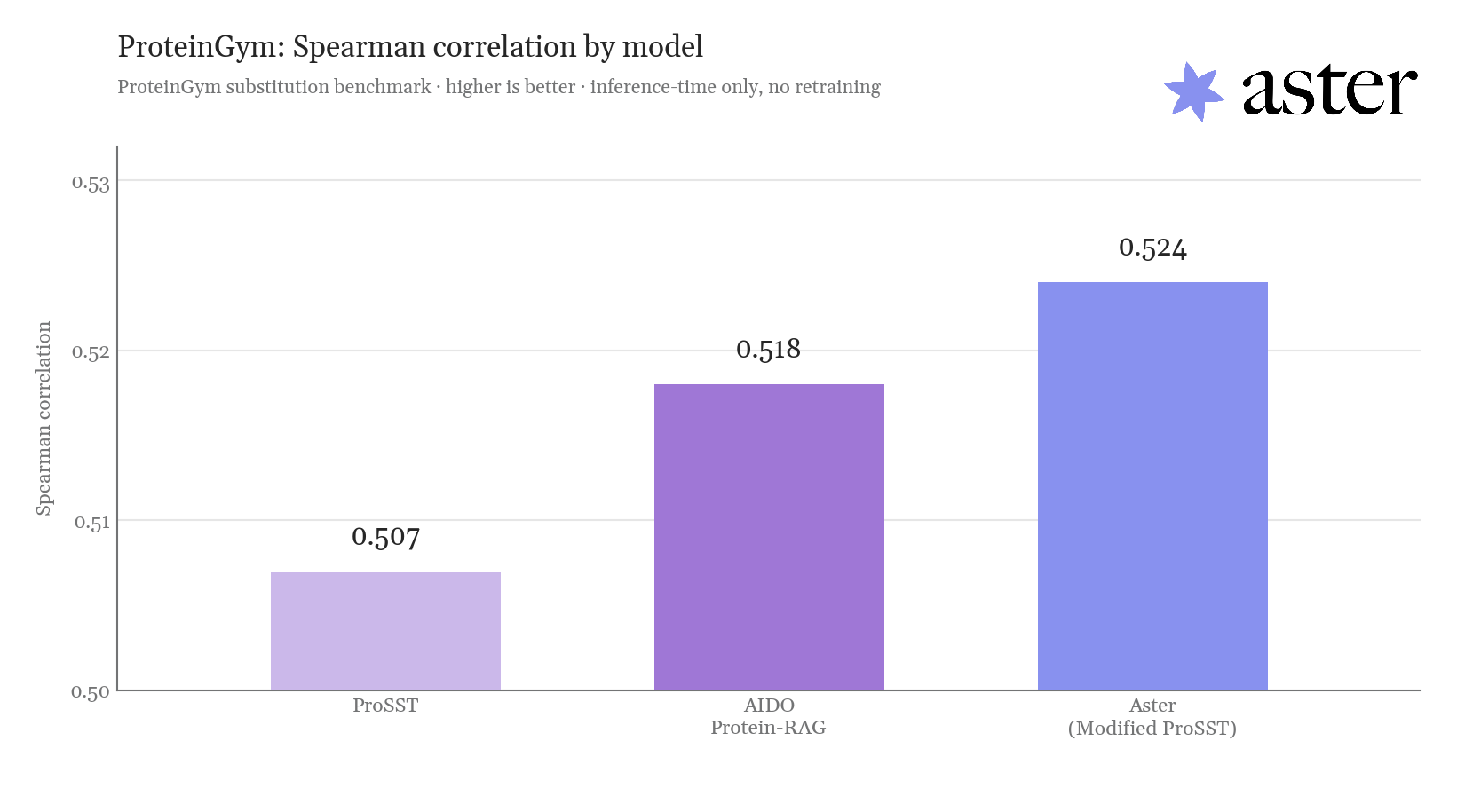
set the record. The final result reached a Spearman correlation of 0.526, with
the single most important change lifting performance from 0.508 to 0.524.
This outperforms the best prior model on the benchmark while being an order of
magnitude faster to inference.
ProteinGym substitution benchmark, Spearman correlation by model (higher is better, inference-time only, no retraining). Aster's modified ProSST reaches 0.524.
We extract the single most simple change that lifts the score from 0.507 to
0.524. It turns out to be a change to the scoring function — from the model's
raw log-probability of a mutation,
si(a)=logpi(a)
to a score that reads the mutation against its position's own distribution:
It is a way to calibrate the model's confidence into the prediction. Because of
its simplicity, this is the only change we consider here — it is the most
interesting scientific example — and it is our submission to the benchmark.
Raw log-likelihood→Confidence-calibrated
#1
L24Iconfident site
model confidence62%top prediction
A
C
D
E
F
G
H
I
K
L
M
N
P
Q
R
S
T
V
W
Y
log p(mut)-3.00
#2
S88Vuncertain site
model confidence10%top prediction
A
C
D
E
F
G
H
I
K
L
M
N
P
Q
R
S
T
V
W
Y
log p(mut)-3.19
Raw log p only sees the mutant’s own probability, so it ranks L24I first. The calibrated score reads each mutant against its position’s whole distribution — folding in the model’s confidence — and the ranking flips. No learned parameters, no tuned weights.
NanoGPT Speedrun
The NanoGPT speedrun is a longstanding machine learning competition. The
objective is to build the fastest program that trains a language model to under
3.28 cross-entropy loss on the FineWeb validation set, using a single node of 8
NVIDIA H100 GPUs.
Progress on this benchmark has produced several important advances in machine
learning, most notably the Muon optimizer.
Three months ago, we applied an earlier version of Aster to set the speedrun
record, against the then-current baseline. When the competition began, training
took 45 minutes; before our
submission, the record stood at 96.8 seconds. Over 8 iterations, Aster shaved
off 1.6 seconds to bring the record to 95.2 seconds.
The solution refined the program's Triton kernels, optimized memory load-ins,
and eliminated unnecessary recomputation.
Closing Thoughts
Each of these results turned work that once took months of human research into a
few hours of autonomous effort. But all three are defined by benchmarks, and
that's where Aster has been successful so far. We believe the next frontier is
open-ended research — problems that elude benchmarks. Solving this will
dramatically expand the range of problems these systems can take on.
Given our current benchmark-driven work, a valid question here is how we'll measure performance once we move to open-ended problems that lack scorable metrics. Currently, we can't measure it directly. However, we believe that benchmarks can serve as proxies for the time being. A system that can push the frontiers of diverse domains such as LLM training, protein prediction, and GPU-kernel speedrunning doesn't necessarily overfit to anything since it's doing something general. That being said, we will push hard on what is measurable while being domain-agnostic, which gives us the strongest available evidence that it will transfer to the open-ended work we ultimately care about.
We're a lean team working on autonomous open-ended research. If you're
interested in working with us, send us an email at
info@asterlab.ai.